Are you a palaeontologist interested in incorporating phylogenetic comparative methods into your research? Would you like to increase your toolkit of hypothesis-testing analyses for fossil-related questions? There’s a pretty good chance you’re going to need a time-calibrated phylogenetic tree. And to get one, you’re going to need to try your hand at R.
If you’re new to R programming or phylogenetic comparative methods, it can seem like a pretty steep uphill battle to learn some of these techniques, especially if you don’t feel like you got a great grounding in programming or statistics as an undergrad. Nevertheless, there are great resources out there for learning the basics of moving around in R (I like this one but I also just google things a lot), and good resources on phylogenetic comparative methods and statistical methods in biology. Today I’m going to do my best to make a bit of a tutorial for an important R package, paleotree (David Bapst), which will make magical time-calibrated trees for you that you can then use for all kinds of wonderful analyses.
What is paleotree? It’s an R package that includes several functions for creating time trees. You should go read Bapst’s extremely excellent blog posts detailing the mechanics and philosophy behind the package, and which is also a very very good tutorial for how to use the package overall. However if, like me, you are a total newbie to R while simultaneously learning how to use this package, you might also do stuff wrong while having limited troubleshooting abilities. That’s where this tutorial comes in. Let’s go!
What do you need to make a time tree in paleotree?
- A phylogenetic tree.
- Information about the ages of the taxa in your tree.
- *Optional: information about the ages of other nodes in your tree (e.g. I had a tree with lots of extant mammals and like 2 fossil taxa; to make the time-calibration make more sense, I needed some ages for deeper splits in the mammal tree, like the split between marsupials and placentals, the split between euarchontoglires and laurasiatheres, etc. Here is an excellent resource for this info if you don’t have it at hand already.)
Formatting your phylogenetic tree:
I work with trees in Mesquite but you may use something different; whatever the case, export your tree as a .tre file rather than a .nex file, because .nex won’t work and will make you sad. Don’t use any special characters in your taxon names like ? or sp. or “Dubious taxon X”. Your taxa should look like Genus_species. When you export the tree, I recommend naming it something really simple to make it less likely to have typos when writing in R, so I often just name my file tree.tre. Original!
Formatting your taxon (tip) age data:
I start by making three columns in Excel: taxon names, maximum age, and minimum age. Taxon names should match the exact order that they appear in your phylogenetic tree data and have the same format, so, Genus_species. Maximum and minimum ages should be pretty self explanatory, but you want to make sure that you don’t get them reversed at any point because then your time tree will not happen. Once you’re all done, save a second copy of this file, and then delete the taxon names column (this means you have less work to do in R later). You can also delete the headers if you want, too. Save this version of the file as a .csv file. As for the tree file, I make my file name really simple, like ranges.csv.
*Formatting your node age data (advanced!)
This one’s a little trickier and is more easily done once your .tre file is already loaded into R, so come back to this later if you need it. You’ll be making a spreadsheet similar to your tip age ranges, but you’re using the internal nodes of the tree rather than the tips. To figure out the numbers for the internal nodes, you can use getMRCA. This finds the most recent common ancestor of two tips on your tree, and you use it like this:
getMRCA(tree,c(“taxonA”,”taxonB”))
Choose the two taxa that bracket your tree, and stick them into the “taxon” sections. R will give you a number that represents the first node at the base of your tree, but it probably won’t be ‘1’, because R labels all of the tips first, then the internal nodes. The best way to format your data is therefore to set up an excel spreadsheet like this: if you have 10 taxa, rows 1-10 in excel are blank, and your first internal node is row 11. Use getMRCA to find the node number for whichever age you want to record, and stick your age into that row in Excel. If you don’t have an age you want to include, you need to fill that row with NA, or else everything will fall apart! Once you’re all finished, you delete rows 1-10, and save as a .csv file.
If you want to double-check nodes, the opposite of getMRCA is getDescendants(tree, node number)
YOU ARE READY FOR RSTUDIO
I like to use RStudio for working with R. You need to do a few things at the beginning of a new session with R:
- Set the working directory, either using setwd, or using the dropdown menu under “Session”. Put all the files you need in the same folder.
- Load your packages. In RStudio, one of the windows will have a ‘packages’ tab where you can check off whatever packages you need for your work. We’ll be using paleotree and phytools. If you don’t have these already, there’s an option to download them from CRAN and it’s super easy.
Reading your files into R is relatively straightforward. First up, read your tree file in:
tree<-read.tree(“tree.tre”)
You can check to make sure your tree looks right by doing
plot(tree)
and if your tree file had multiple trees and you just want to check one, you can call it using
plot(tree[[1]])
You also want to read your time range data in:
ranges<-read.csv(file=”ranges.csv”, header=F, row.names=1)
And your nodes, if you have them:
nodes<-read.csv(file=”nodes.csv”, header=F)
The row.names part is important if you have a column of taxon names, but sometimes things seem to get a bit weird there, so you can use this to make sure everything’s ok
row.names(ranges)<-ranges[,1]
Now is a good time to check to make sure everything is hunky dory with your ranges, because this is where I’ve had some trouble, especially since I was making a time-calibrated tree with hundreds of taxa. It’s easy to mix things up! So, you can check to make sure the names of the ranges and tree line up correctly using
setdiff(ranges[,1],tree$tip.label)
If you get a “character 0” response after using setdiff, you are good to go! If not, try
ranges[,1]<-as.character(ranges[,1])
and check setdiff again.
I had a “ “ show up once while doing this and it was because my range table was including empty rows, so my fix for this was to just copy my range data into a new Excel sheet, resave as a .csv, and read it back into R. Problem solved!
There’s one more thing you need to do to your ranges for paleotree, and that’s to read that information into timeData:
timeData<-ranges=ranges[,2:3]
YOU ARE READY FOR PALEOTREE
Ok, we’ve got our tree/trees, time ranges, and internal node dates read into R and hopefully all talking to each other nicely. We are now ready to use the paleotree function to time-calibrate those trees!
paleotree has three methods for time-scaling your tree, described by David Bapst at his blog and also in the official documentation. With many many many apologies to David because I know cal3TimePaleoPhy is the better method, I have never been able to get my giant dataset of ranges and bins to work properly and in a fit of pique opted to use regular ol’ timePaleoPhy instead, so that’s what I’m going to describe here. It looks like this in the official documentation:
timePaleoPhy(tree, timeData, type=”basic”, vartime=NULL, ntrees=1, randres=FALSE, timeres=FALSE, add.term=FALSE, inc.term.adj=FALSE, dateTreatment=”firstLast”, node.mins=NULL, noisyDrop=TRUE, plot=FALSE)
Hopefully you’ll be able to notice some of the things we’ve already prepared, like tree and timeData! Some of the other options you’ll need to decide for yourself, but I typically use type=”mbl”, vartime=1, ntrees=100 or 500, and dateTreatment=”minMax”. If you have node ages, you’ll want node.mins=”nodes”. If you want to plot your tree, you can set it to plot=TRUE or plot=T.
You’re making a new set of time-calibrated trees, so you’ll write this like so:
tree1<-timePaleoPhy(tree, timeData, type=”basic”, vartime=1, ntrees=100, randres=F, timeres=F, add.term=F, inc.term.adj=F, dateTreatment=”minMax”, node.mins=”nodes”, noisyDrop=T, plot=T)
Hopefully you now have a nice set of time-calibrated trees stored in tree1! You can now save these to your hard drive using
write.nexus(tree1, file=”tree1.nex”)
And that’s it! You can open this file up in Mesquite or figtree if you want to manipulate it there rather than in R, or you can use these trees in other R functions.
The main issues I’ve run into over and over again are problems in the range or node data – it’s really easy to transpose your ranges so that the maximum and minimum ages are reversed, or to mess up the taxon names somehow. Going over your data carefully will reduce a lot of errors, but sometimes these can be hard to spot. Bucky Gates has helpfully created a little bit of code to help find errors in your range data and has graciously allowed me to share it here – download the R file HERE and open it up in R to check it out.
Alright folks, spot any errors in this tutorial? Let me know in the comments and we’ll troubleshoot together!
Huge gigantic thanks for this post go to Bucky Gates, David Bapst, and especially my sister Jessica Arbour who is a total whiz at R and a cool scientist (go check out her papers!) and very patiently walked me through a lot of the problems I outlined here. THANK YOU SMALLER ARBOUR.
*Edited to add a picture because there was an unforgiveable lack of ankylosaurs in this post! Here’s a really cool osteoderm from the indeterminate Albertan ankylosaur ROM 813. The right side shows the exposed bone, but the left side shows the preserved horny sheath impression, and all around it are scale impressions!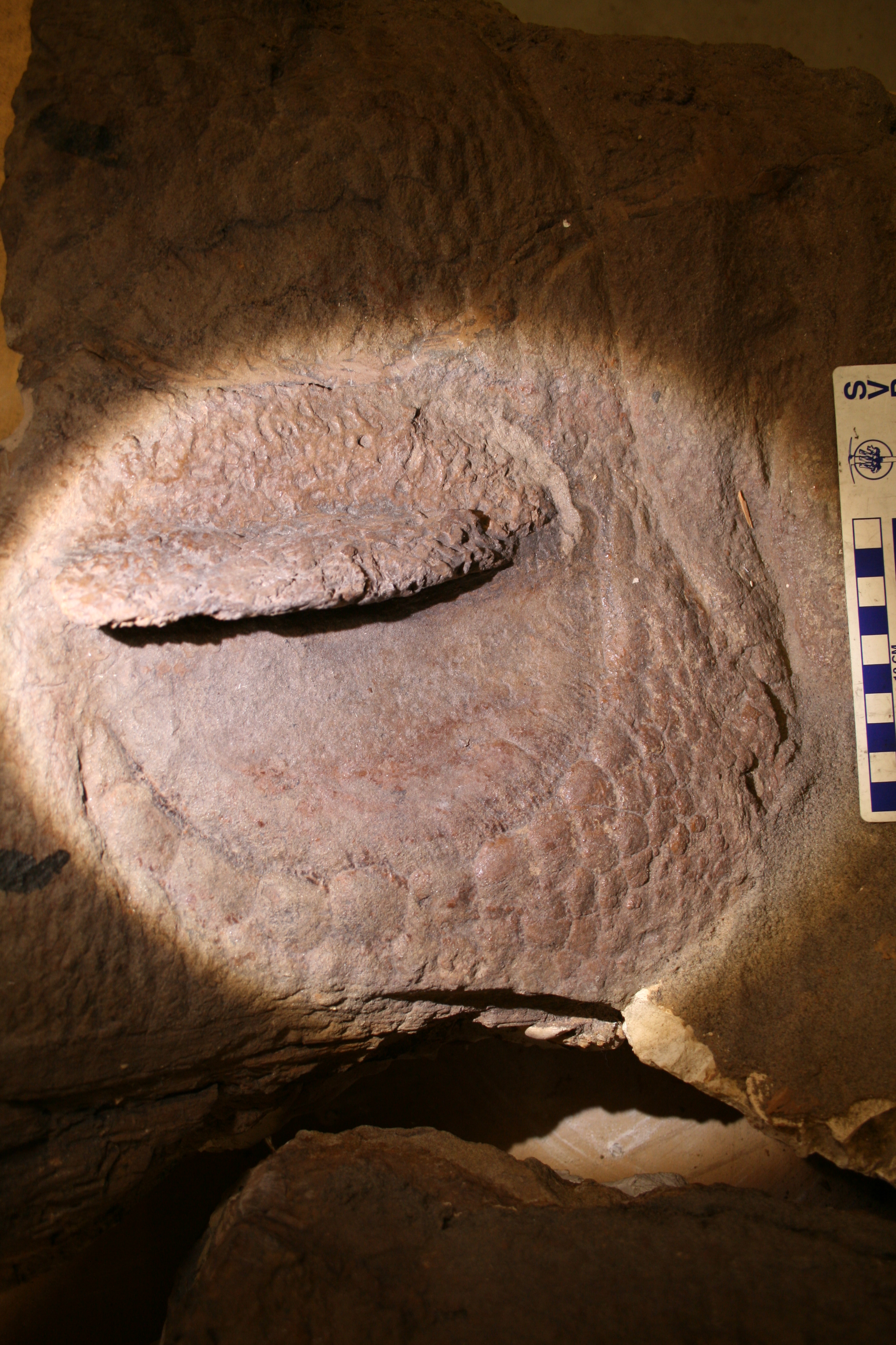

Hi there,
I was just wondering if you know a way to summarize the stochastic trees you obtain in this analysis.
e.g., get one summary tree with the average node ages from the 100 trees contained in your “tree1” object.
Cheers,
LikeLike
Hi Victoria,
Great post, I’m glad to see people using paleotree. And, ah, now I
know Neotropical Cichlid Arbour is related to Ankylosaur Arbour! I
noticed one day I had quite a few Arbour papers in my PDFs folder, and
I had wondered if there was a connection.
Huh, I also didn’t realize there was a need for indicating which taxon
dates were switched; that said, I’ve seen a lot of other, more dire,
issues with time data from users, so I’m not sure that if I had added
the functionality to paleotree to list problematic taxa would help
(other people are having problems like not labeling their data, or
accidentally making their ranges non-numeric, etc). I’m glad Bucky has
already written code to fill that need, though.
So, regarding the use of the dating methods available in timePaleoPhy
(e.g. MBL or equal), my opinion is that I don’t think its right way to
do things, and if you can’t get rate estimates for cal3, and you can’t
use tip-dating methods, than I don’t think the solution is to use
methods we know give bad answers. Rather, I think you should consider
the likely range of estimates for similar groups with similar fossil
records. Then, do cal3 using the end points of those rates to assess
the effect of assuming low/high levels of sampling/diversification
rates on your question of interest (e.g. the result of some
comparative method). I’ve got a lot more to say on this subject, and I
plan to say much more on it soon on my own blog, but for now you
should look at my recent Paleobiology paper with Melanie Hopkins,
which includes a table of sampling rate estimates from various groups.
I admit that my opinion on this has been evolving over many years, but
the fact that using cal3 gives an answer you can’t arrive at even if
you use MBL or ‘equal’ a bunch of different ways, that’s scary. Its
not about which is the ‘better’ method, rather which one works at all.
Cesan, it depends on what you want. There aren’t very good ways
presently to visualize the uncertainty in the dating of the nodes when
topology varies. You can get all the ages for the nodes for a tree
sample with dateNodes, but it will be like drinking from a fire hose
(with good reason). As for the topology alone goes. It may be better
to use the sample of dated trees directly for your question of
interest (e.g. when particular clades diverged, or applying each
comparative method analysis to each tree individually).
I hope the above is helpful,
-Dave
LikeLike